
Mathematik-Online lexicon:
|
|
[home] [lexicon] [problems] [tests] [courses] [auxiliaries] [notes] [staff] |
|
|
Mathematik-Online lexicon: | ||
4-point scheme | ||
| A B C D E F G H I J K L M N O P Q R S T U V W X Y Z | overview |
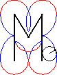
Cubic interpolation is frequently used to fit data ![]() at equally spaced
points
at equally spaced
points ![]() , in particular, for plotting the graph of an interpolating
function
, in particular, for plotting the graph of an interpolating
function ![]() .
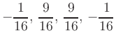
Intermediate values at the midpoints
.
Intermediate values at the midpoints
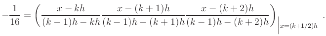
![]() are approximated by a weighted sum of neighboring data:
are approximated by a weighted sum of neighboring data:
![\includegraphics[width=.45\textwidth]{KubischeInterpolation_Bild1}](/inhalt/beispiel/beispiel1/img10.png) |
![\includegraphics[width=.45\textwidth]{KubischeInterpolation_Bild2}](/inhalt/beispiel/beispiel1/img11.png) |
![\includegraphics[width=.45\textwidth]{KubischeInterpolation_Bild3}](/inhalt/beispiel/beispiel1/img12.png) |
![\includegraphics[width=.45\textwidth]{KubischeInterpolation_Bild4}](/inhalt/beispiel/beispiel1/img13.png) |
The figure shows a three-fold application of ![]() -point-interpolation
to data of a sine function.
While the limit function, shown on the left part of the figure,
appears to be smooth, merely the first derivative is continuous.
-point-interpolation
to data of a sine function.
While the limit function, shown on the left part of the figure,
appears to be smooth, merely the first derivative is continuous.
![\includegraphics[width=.4\textwidth]{fourpoint_lim}](/inhalt/beispiel/beispiel1/img14.png)
![\includegraphics[width=.4\textwidth]{fourpoint_diff}](/inhalt/beispiel/beispiel1/img15.png)
The right part of the figure shows an approximation of the second
derivative via divided differences after ![]() -fold interpolation.
Apparently, the graph has a fractal character.
-fold interpolation.
Apparently, the graph has a fractal character.
| automatisch erstellt am 22. 6. 2016 |